Sensitividad FAST

The method

Our goal was to run a sensitivity analysis on the output of an ensemble model

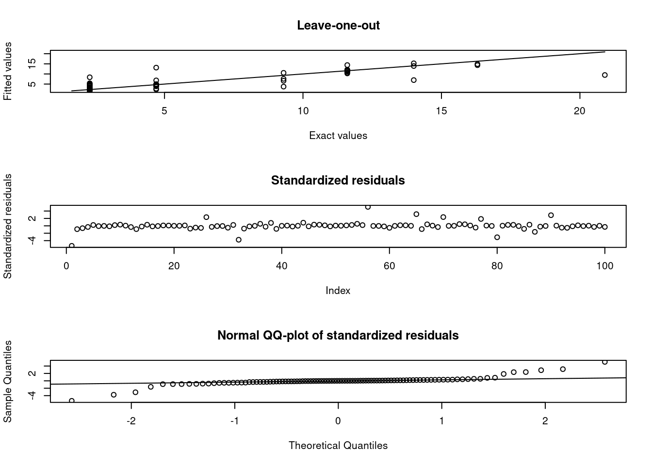
First we built a kriging model, which estimates parameters through maximum likelihood, with function DiceKriging::km(), the model output was used for building a latin hypercube emulator, which was then fed to the Fourier Amplitude Sensitivity Test.

The kriging model

Output from DiceKriging::km()

fit_grd

Call:
km(formula = ~., design = cuiki[, -6], response = cuiki$grdOEMcaByTSS)

Trend  coeff.:
               Estimate
 (Intercept)    48.6827
      biovii    -1.3164
       bioxv    -0.1230
     conddem     0.0005
       dorpc     0.0052
         hft     0.0094
         ire    -0.2230
     logqvar    17.1641
         ria    -0.0122

Covar. type  : matern5_2 
Covar. coeff.:
                 Estimate
 theta(biovii)     0.4009
  theta(bioxv)     1.6833
theta(conddem)  3082.3671
  theta(dorpc)   401.0094
    theta(hft)   301.1015
    theta(ire)     0.0000
theta(logqvar)     0.0351
    theta(ria)   212.7240

Variance estimate: 12.22965

plot(fit_grd)

“variance estimate of 17.19 was obtained through function km from package DiceKriging (Roustant et al., 2012)”

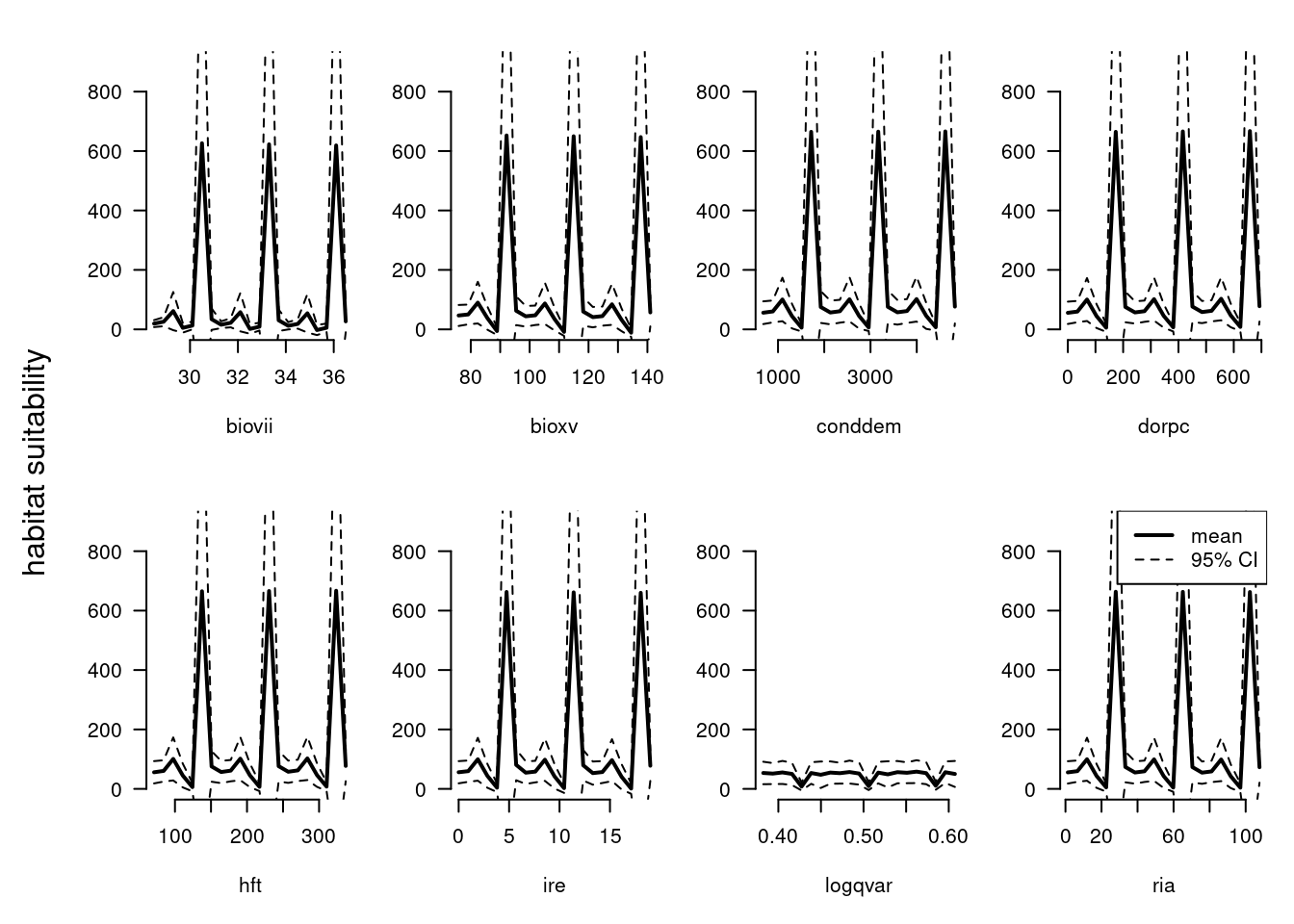
Output from the emulator

n = 21 # number of points in to vary
# (elio) this is the part of the emulator OAAT: "one at a time" variable changing
X_oaat = oaat.design(design=cuiki[,-6], n = n, hold = X.standard)
colnames(X_oaat) = colnames(cuiki[,-6])
# (elio) the model output
pred_grd_oaat = predict(fit_grd, newdata = X_oaat, type = 'UK')

# (elio) plots are almost the same, only logqvar is visibly different
par(mfrow = c(2,4), las = 1, mar = c(5,3,2,1), oma = c(0.1,3,0.1,0.1))
for(i in 1:ncol(X_oaat)){
  # just the points where the parameter varies
  ix <- seq(from = ((i*n) - (n-1)), to =  (i*n), by = 1)
  plot(X_oaat[ix, i], pred_grd_oaat$mean[ix], ylim = c(0, 900), bty = 'n',
       ylab = '', type = 'l', lwd = 2,
       xlab = colnames(cuiki[,-6])[i]
  )
  lines(X_oaat[ix, i], pred_grd_oaat$upper95[ix], lty = 'dashed')
  lines(X_oaat[ix, i], pred_grd_oaat$lower95[ix], lty = 'dashed')
}
legend('topright', lty = c('solid', 'dashed'), lwd = c(2,1), legend = c('mean','95% CI'))
mtext('habitat suitability', side = 2, line = 1, col = 'black', outer = TRUE, las = 0)

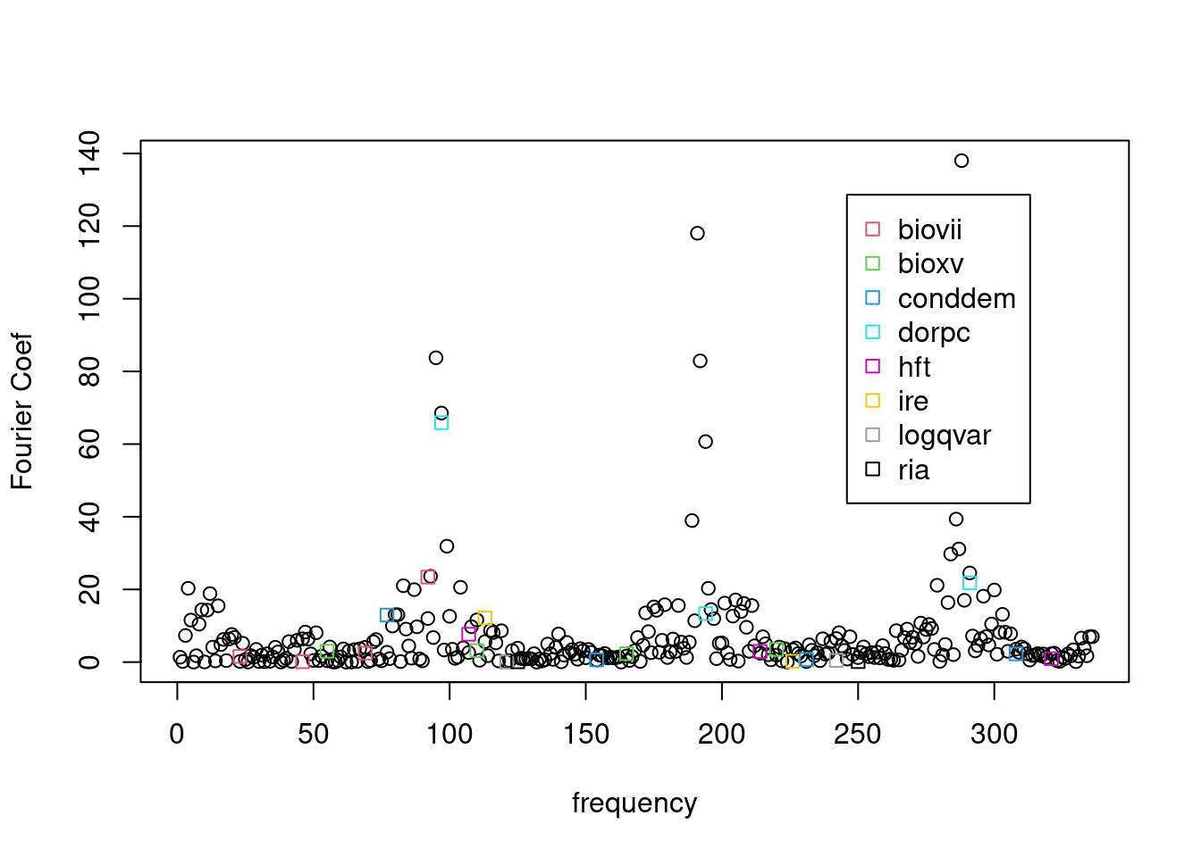
FAST: Fourier amplitude sensitivity test

Here we run the FAST analysis on the pred_grd_oaat object from the emulator. We found the highest fourier coeficients for degree of regulation and bio7

paras = fast_parameters(min = c(27.60000,  75.88765, 308.00000,   0.00000,  63.00000,   0.00000,   0.38227,   0.97400 ),
                max = c(36.5, 140.987823486328, 4825, 693, 337, 19, 0.611429989337921, 245.130996704102))
# (elio) the model needs 243 records (no idea how they came up with that number)
# ...... so I pasted twice the vector
par(mfrow = c(1,1))
fast::sensitivity(c(pred_grd_oaat$mean, pred_grd_oaat$mean), numberf = 8, n = 2, make.plot = T, names = names(cuiki[,-6]))

[1] 6.786656e-03 4.477661e-04 2.121627e-03 6.103061e-02 8.346640e-04
[6] 1.809250e-03 2.875387e-06 3.382124e-07

mtext('fourier coef', side = 2, line = 1, col = 'black', outer = TRUE, las = 0)